Radioactivity

Radioactivity refers to the particles which are emitted from nuclei as a result of nuclear instability. Because the nucleus experiences the intense conflict between the two strongest forces in nature, it should not be surprising that there are many nuclear isotopes which are unstable and emit some kind of radiation. The most common types of radiation are called alpha, beta, and gamma radiation, but there are several other varieties of radioactive decay.

Radioactive decay rates are normally stated in terms of their half-lives, and the half-life of a given nuclear species is related to its radiation risk. The different types of radioactivity lead to different decay paths which transmute the nuclei into other chemical elements. Examining the amounts of the decay products makes possible radioactive dating.

Radiation from nuclear sources is distributed equally in all directions, obeying the inverse square law.

Natural radioactive decay series.

Radioactive items you can buy.

Some history.

Illustration of alpha, beta and gamma radiation

HyperPhysics***** Nuclear

R Nave

Go Back

Alpha Radioactivity

Composed of two protons and two neutrons, the alpha particle is a nucleus of the element helium. Because of its very large mass (more than 7000 times the mass of the beta particle) and its charge, it has a very short range. It is not suitable for radiation therapy since its range is less than a tenth of a millimeter inside the body. Its main radiation hazard comes when it is ingested into the body; it has great destructive power within its short range. In contact with fast-growing membranes and living cells, it is positioned for maximum damage.

Alpha particle emission is modeled as a barrier penetration process. The alpha particle is the nucleus of the helium atom and is the nucleus of highest stability.

Alpha role in deuterium-tritium fusion

Proton fusion

Radioactivity

IndexAlpha particle concepts

HyperPhysics***** Nuclear

R Nave

Alpha Barrier Penetration

The energy of emitted alpha particles was a mystery to early investigators because it was evident that they did not have enough energy, according to classical physics, to escape the nucleus. Once an approximate size of the nucleus was obtained by Rutherford scattering, one could calculate the height of the Coulomb barrier at the radius of the nucleus. It was evident that this energy was several times higher than the observed alpha particle energies. There was also an incredible range of half lives for the alpha particle which could not be explained by anything in classical physics.The resolution of this dilemma came with the realization that there was a finite probability that the alpha particle could penetrate the wall by quantum mechanical tunneling. Using tunneling, Gamow was able to calculate a dependence for the half-life as a function of alpha particle energy which was in agreement with experimental observations.

Modeling of tunneling in polonium

IndexAlpha Decay Concepts

References
Blatt
Ch 15

Tipler
Ch 40

HyperPhysics***** Nuclear

R Nave

Go Back

Alpha Binding Energy

The nuclear binding energy of the alpha particle is extremely high, 28.3 MeV. It is an exceptionally stable collection of nucleons, and those heavier nuclei which can be viewed as collections of alpha particles (carbon-12, oxygen-16, etc.) are also exceptionally stable. This contrasts with a binding energy of only 8 MeV for helium-3, which forms an intermediate step in the proton-proton fusion cycle.

Nuclear units

Index

HyperPhysics***** Nuclear

R Nave

Go Back

Alpha, Beta, and Gamma

Historically, the products of radioactivity were called alpha, beta, and gamma when it was found that they could be analyzed into three distinct species by either a magnetic field or an electric field.

Index

HyperPhysics***** Nuclear

R Nave

Go Back

Penetration of Matter

Though the most massive and most energetic of radioactive emissions, the alpha particle is the shortest in range because of its strong interaction with matter. The electromagnetic gamma ray is extremely penetrating, even penetrating considerable thicknesses of concrete. The electron of beta radioactivity strongly interacts with matter and has a short range.

Index

HyperPhysics***** Nuclear

R Nave

Go Back

History of discovery

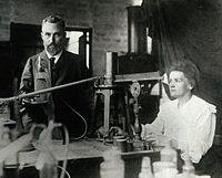
Pierre and Marie Curie in their Paris laboratory, before 1907

Radioactivity was discovered in 1896 by the French scientist Henri Becquerel, while working on phosphorescent materials.^[2] These materials glow in the dark after exposure to light, and he suspected that the glow produced in cathode ray tubes by X-rays might be associated with phosphorescence. He wrapped a photographic plate in black paper and placed various phosphorescent salts on it. All results were negative until he used uranium salts. The result with these compounds was a blackening of the plate. These radiations were called Becquerel Rays.

It soon became clear that the blackening of the plate had nothing to do with phosphorescence, because the plate blackened when the mineral was in the dark. Non-phosphorescent salts of uranium and metallic uranium also blackened the plate. It was clear that there was a form of radiation that could pass through paper and was causing the plate to become black.

At first, it seemed that the new radiation was similar to the then recently discovered X-rays. Further research by Becquerel, Ernest Rutherford, Paul Villard, Pierre Curie, Marie Curie, and others discovered that this form of radioactivity was significantly more complicated. Different types of decay occur, producing very different types of radiation. Rutherford was the first to realize that they all decay in accordance with the same mathematical exponential formula (see below), and Rutherford and his student Frederick Soddy were the first to realize that many decay processes resulted in the transmutation of one element to another. Subsequently, the radioactive displacement law of Fajans and Soddy was formulated to describe the products of alpha and beta decay.

The early researchers also discovered that many other chemical elements besides uranium have radioactive isotopes. A systematic search for the total radioactivity in uranium ores also guided Pierre and Marie Curie to isolate two new elements: polonium and radium. The chemical similarity of radium to barium made these two elements difficult to distinguish, except for the radioactivity of radium.

Early dangers

The dangers of radioactivity and radiation were not immediately recognized. The discovery of x‑rays in 1895 led to widespread experimentation by scientists, physicians, and inventors. Many people began recounting stories of burns, hair loss and worse in technical journals as early as 1896. In February of that year, Professor Daniel and Dr. Dudley of Vanderbilt University performed an experiment involving x-raying Dudley’s head that resulted in him losing his hair under where the tube was placed (reported in the The X-rays Science news supplement). A report by Dr. H.D. Hawks, a graduate of Columbia College, of his suffering severe hand and chest burns in an x-ray demonstration, was the first of many other reports in Electrical Review.^[3] Many experimenters including Elihu Thomson at Thomas Edison’s lab, William J. Morton, and Nikola Tesla also reported burns. Elihu Thomson deliberately exposed a finger to an x-ray tube over a period of time and suffered pain, swelling, and blistering.^[4] Other effects were sometimes blamed for the damage, including ultraviolet rays and (according to Tesla) ozone.^[5] Many physicians claimed that there were no effects from x-ray exposure at all.^[4]

Before the biological effects of radiation were known, many physicians and corporations began marketing radioactive substances as patent medicine in the form of glow-in-the-dark pigments. Examples were radium enema treatments, and radium-containing waters to be drunk as tonics. Marie Curie protested against this sort of treatment, warning that the effects of radiation on the human body were not well understood. Curie later died from aplastic anaemia, likely caused by exposure to ionizing radiation. By the 1930s, after a number of cases of bone necrosis and death of enthusiasts, radium-containing medicinal products had been largely removed from the market (radioactive quackery).

Radiation Protection

Main article: radiation protection

See also: sievert and ionizing radiation

Only a year after Rontgen’s discovery of X rays, the American engineer Wolfram Fuchs (1896) gave what is probably the first protection advice, but it was not until 1925 that the first International Congress of Radiology (ICR) was held and considered establishing international protection standards. The genetic effects of radiation, including the effect of cancer risk, were recognized much later. In 1927, Hermann Joseph Muller published research showing genetic effects and, in 1946, was awarded the Nobel prize for his findings.

The second ICR was held in Stockholm in 1928 and proposed the adoption of the rontgen unit, and the ‘International X-ray and Radium Protection Committee’ (IXRPC) was formed. Rolf Sievert was named Chairman, but a driving force was George Kaye of the British National Physical Laboratory. The committee met at each of the ICR meetings in Paris in 1931, Zurich in 1934, and Chicago in 1937. The first post-war ICR convened in London in 1950, and adopted the present name, the International Commission on Radiological Protection (ICRP).^[6] The ICRP has developed the present international system of radiation protection.

Units of radioactivity

Graphic showing relationships between radioactivity and detected ionizing radiation

The International System of Units (SI) unit of radioactive activity is the becquerel (Bq), named in honour of the scientist Henri Becquerel. One Bq is defined as one transformation (or decay or disintegration) per second.

An older unit of radioactivity is the curie, Ci, which was originally defined as the amount of radium emanation (radon-222) in equilibrium with one gram of pure radium, isotope Ra-226. At present it is equal, by definition, to the activity of any radionuclide decaying with a disintegration rate of 3.7×10¹⁰ Bq, so that 1 curie (Ci) = 3.7×10¹⁰ Bq. For radiological protection purposes, although the United States Nuclear Regulatory Commission permits the use of the unit curie alongside SI units,^[7] the European Union European units of measurement directives required that its use for “public health … purposes” be phased out by 31 December 1985.^[8]

Types of decay

Alpha particles may be completely stopped by a sheet of paper, beta particles by aluminium shielding. Gamma rays can only be reduced by much more substantial mass, such as a very thick layer of lead.

Early researchers found that an electric or magnetic field could split radioactive emissions into three types of beams. The rays were given the alphabetic names alpha, beta, and gamma, in order of their ability to penetrate matter. While alpha decay was seen only in heavier elements (atomic number 52, tellurium, and greater), the other two types of decay were seen in all of the elements. Lead (atomic number 82) is the heaviest element to have any isotopes stable (to the limit of measurement) to radioactive decay. Radioactive decay is seen in all isotopes of all elements of atomic number 83 (bismuth) or greater (bismuth, however, is only very slightly radioactive).

Transition diagram for decay modes of a radionuclide, with neutron number N and atomic number Z (shown are α, β^±, p⁺, and n⁰ emissions, EC denotes electron capture).

Types of radioactive decay related to N and Z numbers

In analysing the nature of the decay products, it was obvious from the direction of electromagnetic forces induced on the radiations by external magnetic and electric fields that alpha particles from decay carried a positive charge, beta particles carried a negative charge, and gamma rays were neutral. From the magnitude of deflection, it was clear that alpha particles were much more massive than beta particles. Passing alpha particles through a very thin glass window and trapping them in a discharge tube allowed researchers to study the emission spectrum of the resulting gas, and ultimately prove that alpha particles are helium nuclei. Other experiments showed the similarity between classical beta radiation and cathode rays: They are both streams of high-speed electrons. Likewise, gamma radiation and X-rays were found to be similar high-energy electromagnetic radiation.

The relationship between the types of decays also began to be examined: For example, gamma decay was almost always found to be associated with other types of decay, and occurred at about the same time, or afterwards. Gamma decay as a separate phenomenon (with its own half-life, now termed isomeric transition), was found in natural radioactivity to be a result of the gamma decay of excited metastable nuclear isomers, which were, in turn, created from other types of decay.

Although alpha, beta, and gamma radiations were most commonly found, other types of decay were eventually discovered. Shortly after the discovery of the positron in cosmic ray products, it was realized that the same process that operates in classical beta decay can also produce positrons (positron emission). In an analogous process, instead of emitting positrons and neutrinos, some proton-rich nuclides were found to capture their own atomic electrons (electron capture), and emit only a neutrino (and usually also a gamma ray). Each of these types of decay involves the capture or emission of nuclear electrons or positrons, and acts to move a nucleus toward the ratio of neutrons to protons that has the least energy for a given total number of nucleons (neutrons plus protons).

A theoretical process of positron capture (analogous to electron capture) is possible in antimatter atoms, but has not been observed since the complex antimatter atoms are not available.^[9] This would require antimatter atoms at least as complex as beryllium-7, which is the lightest known isotope of normal matter to undergo decay by electron capture.

Shortly after the discovery of the neutron in 1932, Enrico Fermi realized that certain rare beta-decay reactions immediately yield neutrons as a decay particle (neutron emission). Isolated proton emission was eventually observed in some elements. It was also found that some heavy elements may undergo spontaneous fission into products that vary in composition. In a phenomenon called cluster decay, specific combinations of neutrons and protons other than alpha particles (helium nuclei) were found to be spontaneously emitted from atoms.

Other types of radioactive decay that emit previously-seen particles were found, but by different mechanisms. An example is internal conversion, which results in electron (and sometimes high-energy photon) emission, even though it involves neither beta nor gamma decay (a neutrino is not emitted, and neither the electron nor photon originate in the nucleus). Internal conversion decay (like isomeric transition gamma decay and neutron emission) involves an excited nuclide releasing energy, without transmutation of one element into another.

Rare events that involve a combination of two beta-decay type events happening simultaneously (see below) are known. Any decay process that does not violate the conservation of energy or momentum laws (and perhaps other particle conservation laws) is permitted to happen, although not all have been detected. An interesting example (discussed in a final section) is bound state beta decay of rhenium-187. In this process, an inverse of electron capture, beta electron-decay of the parent nuclide is not accompanied by beta electron emission, because the beta particle has been captured into the K-shell of the emitting atom. An antineutrino, however, is emitted.

Radionuclides can undergo a number of different reactions. These are summarized in the following table. A nucleus with mass number A and atomic number Z is represented as (A, Z). The column “Daughter nucleus” indicates the difference between the new nucleus and the original nucleus. Thus, (A − 1, Z) means that the mass number is one less than before, but the atomic number is the same as before.

Radioactive decay rates

The decay rate, or activity, of a radioactive substance is characterized by:

Constant quantities:

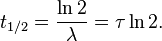
The half-life— $t 1/2$ , is the time taken for the activity of a given amount of a radioactive substance to decay to half of its initial value; see List of nuclides.
The decay constant— $λ$ , “lambda” the inverse of the mean lifetime.
The mean lifetime— $τ$ , “tau” the average lifetime of a radioactive particle before decay.

Although these are constants, they are associated with statistically random behaviour of populations of atoms. In consequence, predictions using these constants are less accurate for small number of atoms.

In principle, the reciprocal of any number greater than one— a half-life, a third-life, or even a (1/√2)-life—can be used in exactly the same way as half-life; but the half-life $t 1/2$ is adopted as the standard time associated with exponential decay.

Time-variable quantities:

Total activity— $A$ , is the number of decays per unit time of a radioactive sample.
Number of particles— $N$ , is the total number of particles in the sample.
Specific activity— $S A$ , number of decays per unit time per amount of substance of the sample at time set to zero (t = 0). “Amount of substance” can be the mass, volume or moles of the initial sample.

These are related as follows:

$t_{1/2} = \frac{\ln(2)}{\lambda} = \tau \ln(2)$

$A = - \frac{\mathrm{d}N}{\mathrm{d}t} = \lambda N$

$S_A a_0 = - \frac{\mathrm{d}N}{\mathrm{d}t}\bigg|_{t=0} = \lambda N_0$

where N₀ is the initial amount of active substance — substance that has the same percentage of unstable particles as when the substance was formed.

Mathematics of radioactive decay

For the mathematical details of exponential decay in general context, see exponential decay.

For related derivations with some further details, see half-life.

For the analogous mathematics in 1st order chemical reactions, see Consecutive reactions.

Universal law of radioactive decay

Radioactivity is one very frequent example of exponential decay. The law describes the statistical behaviour of a large number of nuclides, rather than individual ones. In the following formalism, the number of nuclides or nuclide population N, is of course a discrete variable (a natural number)—but for any physical sample N is so large (amounts of L = 10^23, Avogadro’s constant) that it can be treated as a continuous variable. Differential calculus is needed to set up differential equations for modelling the behaviour of the nuclear decay.

One-decay process

Consider the case of a nuclide $A$ decaying into another $B$ by some process $A \to B$ (emission of other particles, like electron neutrinos ν
e and electrons e^– in beta decay, are irrelevant in what follows). The decay of an unstable nucleus is entirely random and it is impossible to predict when a particular atom will decay.^[1] However, it is equally likely to decay at any time. Therefore, given a sample of a particular radioisotope, the number of decay events $-dN$ expected to occur in a small interval of time $dt$ is proportional to the number of atoms present $N$ , that is^[10]

$-\frac{\mathrm{d}N}{\mathrm{d}t} \propto N.$

Particular radionuclides decay at different rates, so each has its own decay constant $λ$ . The expected decay $-dN/N$ is proportional to an increment of time, $dt$ :

$-\frac{\mathrm{d}N}{N} = \lambda \mathrm{d}t$

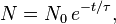
The negative sign indicates that $N$ decreases as time increases, as the decay events follow one after another. The solution to this first-order differential equation is the function:

$N(t) = N_0\,e^{-{\lambda}t} = N_0\,e^{-t/ \tau}, \,\!$

where $N 0$ is the value of $N$ at time $t$ = 0.^[10]

We have for all time $t$ :

$N_A + N_B = N_\mathrm{total} = N_{A0},$

where $N total$ is the constant number of particles throughout the decay process, which is clearly equal to the initial number of $A$ nuclides since this is the initial substance.

If the number of non-decayed $A$ nuclei is:

$N_A = N_{A0}e^{-{\lambda}t} \,\!$

then the number of nuclei of $B$ , i.e. the number of decayed $A$ nuclei, is

$N_B = N_{A0} - N_A = N_{A0} - N_{A0}e^{-{\lambda}t} = N_{A0} \left ( 1 - e^{-{\lambda}t} \right ).$

The number of decays observed over a given interval obeys Poisson statistics. If the average number of decays is $<N>$ , the probability of a given number of decays $N$ is^[10]

$P(N) = \frac{\langle N \rangle^N \exp(-\langle N\rangle)}{N!} .$

Chain-decay processes

Chain of two decays

Now consider the case of a chain of two decays: one nuclide $A$ decaying into another $B$ by one process, then $B$ decaying into another $C$ by a second process, i.e. $A \to B \to C$ . The previous equation cannot be applied to the decay chain, but can be generalized as follows. Since $A$ decays into $B$ , then $B$ decays into $C$ , the activity of $A$ adds to the total number of $B$ nuclides in the present sample, before those $B$ nuclides decay and reduce the number of nuclides leading to the later sample. In other words, the number of second generation nuclei $B$ increases as a result of the first generation nuclei decay of $A$ , and decreases as a result of its own decay into the third generation nuclei $C$ .^[11] The sum of these two terms gives the law for a decay chain for two nuclides:

$\frac{\mathrm{d}N_B}{\mathrm{d}t} = -\lambda_B N_B + \lambda_A N_A.$

The rate of change of $N B$ , that is $dN B /dt$ , is related to the changes in the amounts of $A$ and $B$ , $N B$ can increase as $B$ is produced from $A$ and decrease as $B$ produces $C$ .

Re-writing using the previous results:

$\frac{\mathrm{d}N_B}{\mathrm{d}t} = - \lambda_B N_B + \lambda_A N_{A0} e^{-\lambda_A t}$

The subscripts simply refer to the respective nuclides, i.e. $N A$ is the number of nuclides of type $A$ , $N A0$ is the initial number of nuclides of type $A$ , $λ A$ is the decay constant for $A$ – and similarly for nuclide $B$ . Solving this equation for $N B$ gives:

$N_B = \frac{N_{A0}\lambda_A}{\lambda_B - \lambda_A} \left ( e^{-\lambda_A t} - e^{-\lambda_B t}\right ) .$

Naturally, in the case where $B$ is a stable nuclide ( $λ B$ = 0), this equation reduces to the previous solution, in the case :

$\lim_{\lambda_B\rightarrow 0} \left [ \frac{N_{A0}\lambda_A}{\lambda_B - \lambda_A} \left ( e^{-\lambda_A t} - e^{-\lambda_B t}\right ) \right ] = \frac{N_{A0}\lambda_A}{0 - \lambda_A} \left ( e^{-\lambda_A t} - 1 \right ) = N_{A0} \left ( 1- e^{-\lambda_A t} \right ),$

as shown above for one decay. The solution can be found by the integration factor method, where the integrating factor is $e λ B t$ . This case is perhaps the most useful, since it can derive both the one-decay equation (above) and the equation for multi-decay chains (below) more directly.

Chain of any number of decays

For the general case of any number of consecutive decays in a decay chain, i.e. $A 1 \to A 2 \cdot\cdot\cdot \to A i \cdot\cdot\cdot \to A D$ , where $D$ is the number of decays and $i$ is a dummy index ( $i = 1, 2, 3, \dotsD$ ), each nuclide population can be found in terms of the previous population. In this case $N 2 = 0$ , $N 3 = 0$ ,…, $N D = 0$ . Using the above result in a recursive form:

$\frac{\mathrm{d}N_j}{\mathrm{d}t} = - \lambda_j N_j + \lambda_{j-1} N_{(j-1)0} e^{-\lambda_{j-1} t}.$

The general solution to the recursive problem is given by Bateman’s equations:^[12]

Bateman’s equations $N_D = \frac{N_1(0)}{\lambda_D} \sum_{i=1}^D \lambda_i c_i e^{-\lambda_i t}$ $c_i = \prod_{j=1, i\neq j}^D \frac{\lambda_j}{\lambda_j - \lambda_i}$

Alternative decay modes

In all of the above examples, the initial nuclide decays into only one product.^[13] Consider the case of one initial nuclide that can decay into either of two products, that is $A \to B$ and $A \to C$ in parallel. For example, in a sample of potassium-40, 89.3% of the nuclei decay to calcium-40 and 10.7% to argon-40. We have for all time $t$ :

$N = N_A + N_B + N_C$

which is constant, since the total number of nuclides remains constant. Differentiating with respect to time:

$\begin{align} \frac{\mathrm{d}N_A}{\mathrm{d}t} & = - \left(\frac{\mathrm{d}N_B}{\mathrm{d}t} + \frac{\mathrm{d}N_C}{\mathrm{d}t} \right) \\ - \lambda N_A & = - N_A \left ( \lambda_B + \lambda_C \right ) \\ \end{align}$

defining the total decay constant $λ$ in terms of the sum of partial decay constants $λ B$ and $λ C$ :

$\lambda = \lambda_B + \lambda_C .$

Notice that

$\frac{\mathrm{d}N_A}{\mathrm{d}t} < 0,\frac{\mathrm{d}N_B}{\mathrm{d}t} > 0, \frac{\mathrm{d}N_C}{\mathrm{d}t} > 0. $

Solving this equation for $N A$ :

$N_A = N_{A0} e^{-\lambda t} .$

where $N A0$ is the initial number of nuclide A. When measuring the production of one nuclide, one can only observe the total decay constant $λ$ . The decay constants $λ B$ and $λ C$ determine the probability for the decay to result in products $B$ or $C$ as follows:

$N_B = \frac{\lambda_B}{\lambda} N_{A0} \left ( 1 - e^{-\lambda t} \right ),$

$N_C = \frac{\lambda_C}{\lambda} N_{A0} \left ( 1 - e^{-\lambda t} \right ).$

because the fraction $λ B /λ$ of nuclei decay into $B$ while the fraction $λ C /λ$ of nuclei decay into $C$ .

Corollaries of the decay laws

The above equations can also be written using quantities related to the number of nuclide particles $N$ in a sample;

The activity: $A = λN.$
The amount of substance: $n = N/L$ .
The mass: $M = A r n = A r N/L$ .

where L = 6.022×10²³ is Avogadro’s constant, $A r$ is the relative atomic mass number, and the amount of the substance is in moles.

Decay timing: definitions and relations

Time constant and mean-life

For the one-decay solution $A \to B$ :

$N = N_0\,e^{-{\lambda}t} = N_0\,e^{-t/ \tau}, \,\!$

the equation indicates that the decay constant $λ$ has units of $t -1$ , and can thus also be represented as 1/ $τ$ , where $τ$ is a characteristic time of the process called the time constant.

In a radioactive decay process, this time constant is also the mean lifetime for decaying atoms. Each atom “lives” for a finite amount of time before it decays, and it may be shown that this mean lifetime is the arithmetic mean of all the atoms’ lifetimes, and that it is $τ$ , which again is related to the decay constant as follows:

$\tau = \frac{1}{\lambda}.$

This form is also true for two-decay processes simultaneously $A \to B + C$ , inserting the equivalent values of decay constants (as given above)

$\lambda = \lambda_B + \lambda_C \,$

into the decay solution leads to:

$\frac{1}{\tau} = \lambda = \lambda_B + \lambda_C = \frac{1}{\tau_B} + \frac{1}{\tau_C}\,$

Simulation of many identical atoms undergoing radioactive decay, starting with either 4 atoms (left) or 400 (right). The number at the top indicates how many half-lives have elapsed. Note the law of large numbers: with more atoms, the overall decay is less random.

Half-life

A more commonly used parameter is the half-life. Given a sample of a particular radionuclide, the half-life is the time taken for half the radionuclide’s atoms to decay. For the case of one-decay nuclear reactions:

$N = N_0\,e^{-{\lambda}t} = N_0\,e^{-t/ \tau}, \,\!$

the half-life is related to the decay constant as follows: set $N = N 0 /2$ and $t$ = $T 1/2$ to obtain

$t_{1/2} = \frac{\ln 2}{\lambda} = \tau \ln 2.$

This relationship between the half-life and the decay constant shows that highly radioactive substances are quickly spent, while those that radiate weakly endure longer. Half-lives of known radionuclides vary widely, from more than 10¹⁹ years, such as for the very nearly stable nuclide ²⁰⁹Bi, to 10⁻²³ seconds for highly unstable ones.

The factor of $ln(2)$ in the above relations results from the fact that concept of “half-life” is merely a way of selecting a different base other than the natural base $e$ for the lifetime expression. The time constant $τ$ is the e -1 -life, the time until only 1/e remains, about 36.8%, rather than the 50% in the half-life of a radionuclide. Thus, $τ$ is longer than $t 1/2$ . The following equation can be shown to be valid:

$N(t) = N_0\,e^{-t/ \tau} =N_0\,2^{-t/t_{1/2}}. \,\!$

Since radioactive decay is exponential with a constant probability, each process could as easily be described with a different constant time period that (for example) gave its “(1/3)-life” (how long until only 1/3 is left) or “(1/10)-life” (a time period until only 10% is left), and so on. Thus, the choice of $τ$ and $t 1/2$ for marker-times, are only for convenience, and from convention. They reflect a fundamental principle only in so much as they show that the same proportion of a given radioactive substance will decay, during any time-period that one chooses.

Mathematically, the $n th$ life for the above situation would be found in the same way as above—by setting $N = N 0 /n$ , ${{{1}}}$ and substituting into the decay solution to obtain

$t_{1/n} = \frac{\ln n}{\lambda} = \tau \ln n.$

Example

A sample of ¹⁴C, whose half-life is 5,730 years, has a decay rate of 14 disintegration per minute (dpm) per gram of natural carbon. An artefact is found to have radioactivity of 4 dpm per gram of its present C, how old is the artefact?

Using the above equation, we have:

$N = N_0\,e^{-t/ \tau},$

where: $\frac{N}{ N_0} = 4/14 \approx 0.286,$

$\tau = \frac{T_{1/2}}{\ln 2} \approx 8267$ years,

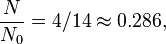
$t = -\tau\,\ln\frac{N}{ N_0} \approx 10360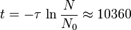$ years.

Changing decay rates

The radioactive decay modes of electron capture and internal conversion are known to be slightly sensitive to chemical and environmental effects that change the electronic structure of the atom, which in turn affects the presence of 1s and 2s electrons that participate in the decay process. A small number of mostly light nuclides are affected. For example, chemical bonds can affect the rate of electron capture to a small degree (in general, less than 1%) depending on the proximity of electrons to the nucleus. In ⁷Be, a difference of 0.9% has been observed between half-lives in metallic and insulating environments.^[14] This relatively large effect is because beryllium is a small atom whose valence electrons are in 2s atomic orbitals, which are subject to electron capture in ⁷Be because (like all s atomic orbitals in all atoms) they naturally penetrate into the nucleus.

In 1992, Jung et al. of the Darmstadt Heavy-Ion Research group observed an accelerated β decay of ¹⁶³Dy⁶⁶⁺. Although neutral ¹⁶³Dy is a stable isotope, the fully ionized ¹⁶³Dy⁶⁶⁺ undergoes β decay into the K and L shells with a half-life of 47 days.^[15]

Rhenium-187 is another spectacular example. ¹⁸⁷Re normally beta decays to ¹⁸⁷Os with a half-life of 41.6 × 10⁹ years,^[16] but studies using fully ionised ¹⁸⁷Re atoms (bare nuclei) have found that this can decrease to only 33 years. This is attributed to “bound-state β⁻ decay” of the fully ionised atom – the electron is emitted into the “K-shell” (1s atomic orbital), which cannot occur for neutral atoms in which all low-lying bound states are occupied.^[17]

Decay Rate of Radon-222 as a function of date and time of day. The color-bar gives the power of the observed signal and represents ~4% seasonal decay rate variation.

A number of experiments have found that decay rates of other modes of artificial and naturally occurring radioisotopes are, to a high degree of precision, unaffected by external conditions such as temperature, pressure, the chemical environment, and electric, magnetic, or gravitational fields.^[18] Comparison of laboratory experiments over the last century, studies of the Oklo natural nuclear reactor (which exemplified the effects of thermal neutrons on nuclear decay), and astrophysical observations of the luminosity decays of distant supernovae (which occurred far away so the light has taken a great deal of time to reach us), for example, strongly indicate that unperturbed decay rates have been constant (at least to within the limitations of small experimental errors) as a function of time as well.

Recent results suggest the possibility that decay rates might have a weak dependence on environmental factors. It has been suggested that measurements of decay rates of silicon-32, manganese-54, and radium-226 exhibit small seasonal variations (of the order of 0.1%),^[19]^[20]^[21] while the decay of Radon-222 exhibit large 4% peak-to-peak seasonal variations,^[22] proposed to be related to either solar flare activity or distance from the Sun. However, such measurements are highly susceptible to systematic errors, and a subsequent paper^[23] has found no evidence for such correlations in seven other isotopes (²²Na, ⁴⁴Ti, ¹⁰⁸Ag, ¹²¹Sn, ¹³³Ba, ²⁴¹Am, ²³⁸Pu), and sets upper limits on the size of any such effects.

Theoretical basis of decay phenomena

The neutrons and protons that constitute nuclei, as well as other particles that approach close enough to them, are governed by several interactions. The strong nuclear force, not observed at the familiar macroscopic scale, is the most powerful force over subatomic distances. The electrostatic force is almost always significant, and, in the case of beta decay, the weak nuclear force is also involved.

The interplay of these forces produces a number of different phenomena in which energy may be released by rearrangement of particles in the nucleus, or else the change of one type of particle into others. These rearrangements and transformations may be hindered energetically, so that they do not occur immediately. In certain cases, random quantum vacuum fluctuations are theorized to promote relaxation to a lower energy state (the “decay”) in a phenomenon known as quantum tunneling. Radioactive decay half-life of nuclides has been measured over timescales of 55 orders of magnitude, from 2.3 x 10⁻²³ seconds (for hydrogen-7) to 6.9 x 10³¹ seconds (for tellurium-128).^[24] The limits of these timescales are set by the sensitivity of instrumentation only, and there are no known natural limits to how brief or long a decay half life for radioactive decay of a radionuclide may be.

The decay process, like all hindered energy transformations, may be analogized by a snowfield on a mountain. While friction between the ice crystals may be supporting the snow’s weight, the system is inherently unstable with regard to a state of lower potential energy. A disturbance would thus facilitate the path to a state of greater entropy: The system will move towards the ground state, producing heat, and the total energy will be distributable over a larger number of quantum states. Thus, an avalanche results. The total energy does not change in this process, but, because of the second law of thermodynamics, avalanches have only been observed in one direction and that is toward the “ground state” — the state with the largest number of ways in which the available energy could be distributed.

Such a collapse (a decay event) requires a specific activation energy. For a snow avalanche, this energy comes as a disturbance from outside the system, although such disturbances can be arbitrarily small. In the case of an excited atomic nucleus, the arbitrarily small disturbance comes from quantum vacuum fluctuations. A radioactive nucleus (or any excited system in quantum mechanics) is unstable, and can, thus, spontaneously stabilize to a less-excited system. The resulting transformation alters the structure of the nucleus and results in the emission of either a photon or a high-velocity particle that has mass (such as an electron, alpha particle, or other type).

Occurrence and applications

According to the Big Bang theory, stable isotopes of the lightest five elements (H, He, and traces of Li, Be, and B) were produced very shortly after the emergence of the universe, in a process called Big Bang nucleosynthesis. These lightest stable nuclides (including deuterium) survive to today, but any radioactive isotopes of the light elements produced in the Big Bang (such as tritium) have long since decayed. Isotopes of elements heavier than boron were not produced at all in the Big Bang, and these first five elements do not have any long-lived radioisotopes. Thus, all radioactive nuclei are, therefore, relatively young with respect to the birth of the universe, having formed later in various other types of nucleosynthesis in stars (in particular, supernovae), and also during ongoing interactions between stable isotopes and energetic particles. For example, carbon-14, a radioactive nuclide with a half-life of only 5,730 years, is constantly produced in Earth’s upper atmosphere due to interactions between cosmic rays and nitrogen.

Nuclides that are produced by radioactive decay are called radiogenic nuclides, whether they themselves are stable or not. There exist stable radiogenic nuclides that were formed from short-lived extinct radionuclides in the early solar system.^[25]^[26] The extra presence of these stable radiogenic nuclides (such as Xe-129 from primordial I-129) against the background of primordial stable nuclides can be inferred by various means.

Radioactive decay has been put to use in the technique of radioisotopic labeling, which is used to track the passage of a chemical substance through a complex system (such as a living organism). A sample of the substance is synthesized with a high concentration of unstable atoms. The presence of the substance in one or another part of the system is determined by detecting the locations of decay events.

On the premise that radioactive decay is truly random (rather than merely chaotic), it has been used in hardware random-number generators. Because the process is not thought to vary significantly in mechanism over time, it is also a valuable tool in estimating the absolute ages of certain materials. For geological materials, the radioisotopes and some of their decay products become trapped when a rock solidifies, and can then later be used (subject to many well-known qualifications) to estimate the date of the solidification. These include checking the results of several simultaneous processes and their products against each other, within the same sample. In a similar fashion, and also subject to qualification, the rate of formation of carbon-14 in various eras, the date of formation of organic matter within a certain period related to the isotope’s half-life may be estimated, because the carbon-14 becomes trapped when the organic matter grows and incorporates the new carbon-14 from the air. Thereafter, the amount of carbon-14 in organic matter decreases according to decay processes that may also be independently cross-checked by other means (such as checking the carbon-14 in individual tree rings, for example).

Origins of radioactive nuclides

Main article: nucleosynthesis

Radioactive primordial nuclides found in the Earth are residues from ancient supernova explosions which occurred before the formation of the solar system. They are the long-lived fraction of radionuclides surviving in the primordial solar nebula through planet accretion until the present. The naturally occurring short-lived radiogenic radionuclides found in rocks are the daughters of these radioactive primordial nuclides. Another minor source of naturally occurring radioactive nuclides are cosmogenic nuclides, formed by cosmic ray bombardment of material in the Earth’s atmosphere or crust. The radioactive decay of these radionuclides in rocks within Earth’s mantle and crust contribute significantly to Earth’s internal heat budget

REVIEW QUESTION

1. EXPLAIN THE DISCOVERY OF RADIOACTIVITY

2. WHAT IS RADIOACTIVE

3. WHAT ARE RADIOACTIVE ELEMENT

4. EXPLAIN THE HALF LIFE OF A RADIO ACTIVE ELEMENT

5. DECAY CONSTANT

6. WHAT ARE THE TYPE OF RADIOACTIVITY

7. RADIO ISOTOPES

8. EXPLAIN THE TERM BOMBARDING

sciencejoint

BRING SCIENCE TO LIFE

RADIOACTIVITY

Radioactivity

Alpha Radioactivity

Alpha Barrier Penetration

Alpha Binding Energy

Alpha, Beta, and Gamma

Penetration of Matter

History of discovery

Early dangers

Radiation Protection

Units of radioactivity

Types of decay

Radioactive decay rates

Mathematics of radioactive decay

Universal law of radioactive decay

One-decay process

Chain-decay processes

Alternative decay modes

Corollaries of the decay laws

Decay timing: definitions and relations

Time constant and mean-life

Half-life

Example

Changing decay rates

Theoretical basis of decay phenomena

Occurrence and applications

Origins of radioactive nuclides

Leave a comment Cancel reply

Radioactivity

Alpha Radioactivity

Alpha Barrier Penetration

Alpha Binding Energy

Alpha, Beta, and Gamma

Penetration of Matter

History of discovery

Early dangers

Radiation Protection

Units of radioactivity

Types of decay

Radioactive decay rates

Mathematics of radioactive decay

Universal law of radioactive decay

One-decay process

Chain-decay processes

Alternative decay modes

Corollaries of the decay laws

Decay timing: definitions and relations

Time constant and mean-life

Half-life

Example

Changing decay rates

Theoretical basis of decay phenomena

Occurrence and applications

Origins of radioactive nuclides

Share this:

Related

Leave a comment Cancel reply